Performing Multi-label Text Classification with Keras

July 31, 2018

Machine Learning

Text classification is a common task where machine learning is applied. Be it questions on a Q&A platform, a support request, an insurance claim or a business inquiry - all of these are usually written in free form text and use vocabulary which might be specific to a certain field. This article demonstrates how such classification problems can be tackled with the open source neural network library Keras.

Analysis of the Cross Validated Dataset

There are various question and answer platforms where people ask an expert community of volunteers for explanations or answers to their questions. One of these platforms is Cross Validated, a Q&A platform for "people interested in statistics, machine learning, data analysis, data mining, and data visualization" (stats.stackexchange.com). Just like on Stackoverflow and other sites which belong to Stackexchange, questions are tagged with keywords to improve discoverability for people who have got expertise in fields indicated by these keywords.

Approximately 85000 such questions have been published as a dataset on kaggle.com. Given this dataset we trained a Keras model which predicts keywords for new questions.
The 85000 questions are labelled with a total of approximately 244000 labels. There are 1315 unique tags in this dataset.

tag frequency

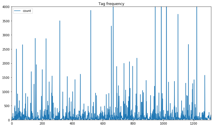
The plot above shows the count for each tag, cropped at 4000 occurrences. This clearly shows that some tags are over-represented while others are assigned to only a few questions. This is an instance of the Class Imbalance Problem which needs to be addressed in the data preparation and model training phase.

Dataset Preparation

The 2017 Kaggle survey lists "dirty data" as a main challenge for practitioners. The advent of deep learning reduced the time needed for feature engineering, as many features can be learned by neural networks. However data preparation and feature engineering remain very important tasks. (cf. deep learning with python))

The Cross Validated dataset only required a few preparation steps. We stripped HTML tags from the question bodies before tokenization and removed tags with a low number of questions.

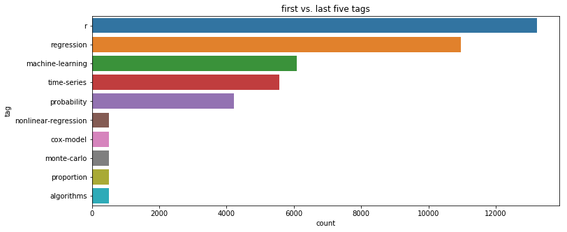
Reducing the Problem to the Most Common Tags in the Dataset

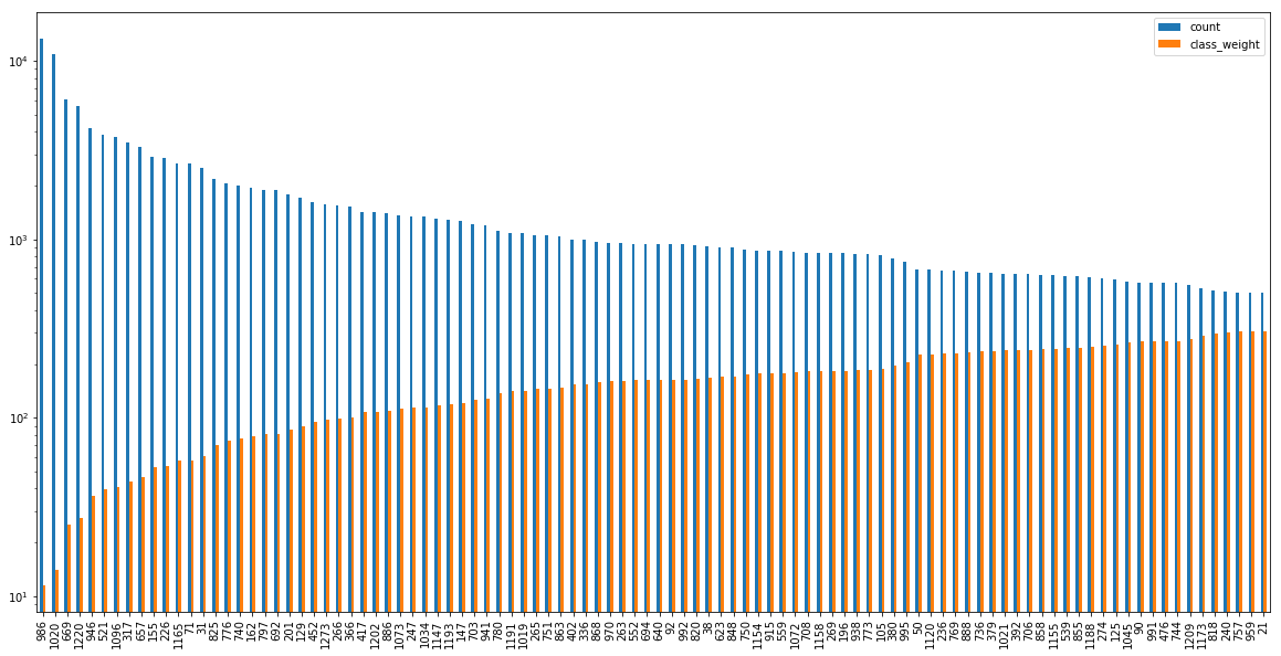
For rare tags there were simply not enough samples available to get reliable results, thus only the top 100 tags were kept. But even with only the 100 most frequently used tags there is still an imbalance as some tags are used more often than others.

first vs last 5 tags

To address this imbalance we calculated class weights to be used as parameters for the loss function of our model. By multiplying the class weights with the categorical losses we can counter the imbalance, so that making false classifications for the tag algorithms is equally expensive as for the tag r.
The calculated class weights are plotted against the counts of the tags below.

class weights plotted vs class observations

There are alternative ways to address class imbalances. We could also have used resampling to duplicate samples in under-represented classes or reduce the number of samples in over-represented classes or trained several models with balanced subsets of the data and model averaging. (cf. Longadge2013) For resampling there is a scikit-learn compatible library imbalanced-learn which also illustrates the class imbalance problem and supported resampling strategies in its documentation.

Cleaning and Tokenizing the Text

The question body contains HTML tags that we don't want to feed into our model. We stripped all HTML tags and combined title and question body into a single field for simplicity.
Note that modelling the neural network with two inputs - one for the title, one for the body - might result in higher accuracy when the title already carries the most important information and the body just adds noise. In such a case the model could learn that the title is more important than the body text.

Tokenization splits a text into tokens (usually individual words), these can then be represented as numbers so that they can be used as feature-vectors for machine learning. Scikit-learn provides a CountVectorizer and a TfidfVectorizer to vectorize text. Keras also comes with several text preprocessing classes - one of these classes is the Tokenizer, which we used for preprocessing.

from keras.preprocessing.text import Tokenizer
from keras.preprocessing.sequence import pad_sequences

tokenizer = Tokenizer(num_words=5000, lower=True)
tokenizer.fit_on_texts(df_questions.Text)
sequences = tokenizer.texts_to_sequences(df_questions.Text)
x = pad_sequences(sequences, maxlen=180)

In the snippet above only the most frequent 5000 words are used to build a dictionary. We limit the sequence length to 180 words.

The labels need to be encoded as well, so that the 100 labels will be represented as 100 binary elements in an array. This was done with the MultiLabelBinarizer from the sklearn library.

from sklearn.preprocessing import MultiLabelBinarizer

multilabel_binarizer = MultiLabelBinarizer()
multilabel_binarizer.fit(df_questions.Tags)
y = multilabel_binarizer.classes_

Finally we can split our data into training and test set to conclude the data preparation:

from sklearn.model_selection import train_test_split

x_train, x_test, y_train, y_test = train_test_split(x, y, test_size=0.2, random_state=9000)

Model Creation

There are various approaches to classify text and in practice you should try several of them to see which one works best for the task at hand. For brevity we will focus on Keras in this article, but we encourage you to try LightGBM, Support Vector Machines or Logistic Regression with n-grams or tf-idf input features. The latter shallow classifiers can be created as binary classifiers - one for each category. By running all of them one can determine probabilities for each category. Sklearn comes with the OneVsRestClassifier which supports this strategy. This is briefly demonstrated in our notebook multi-label classification with sklearn on Kaggle which you may use as a starting point for further experimentation.

Word Embeddings

In the previous steps we tokenized our text and vectorized the resulting tokens using one-hot encoding. The resulting vectors are sparse, binary representations which mainly contain zeros and are high-dimensional (depending on the number of unique words in the vocabulary).

Word embeddings on the other hand are low dimensional as they represent tokens as dense floating point vectors and thus pack more information into fewer dimensions. Words with similar meanings are associated with similar representations. Word embeddings can be obtained in two ways:

Learn word embeddings together with the weights of the neural network
Load pretrained word embeddings which were precomputed as part of a different machine learning task.

We decided to learn new word embeddings as the dataset contains vocabulary which is specific to the domain of statistics and we didn't expect to benefit from pretrained embeddings which use a broader vocabulary.

Simple Baseline

We started with a simple model which only consists of an embedding layer, a dropout layer to reduce the size and prevent overfitting, a max pooling layer and one dense layer with a sigmoid activation to produce probabilities for each of the 100 classes that we want to predict.

from keras.models import Sequential
from keras.layers import Dense, Embedding, GlobalMaxPool1D, Dropout
from keras.optimizers import Adam

model = Sequential()
model.add(Embedding(max_words, 20, input_length=maxlen))
model.add(Dropout(0.15))
model.add(GlobalMaxPool1D())
model.add(Dense(num_classes, activation='sigmoid'))

model.compile(optimizer=Adam(0.015), loss='binary_crossentropy', metrics=['categorical_accuracy'])
callbacks = [
    ReduceLROnPlateau(),
    EarlyStopping(patience=4),
    ModelCheckpoint(filepath='model-simple.h5', save_best_only=True)
]

history = model.fit(x_train, y_train,
                    class_weight=class_weight,
                    epochs=20,
                    batch_size=32,
                    validation_split=0.1
                    callbacks=callbacks)

With this simple model the categorical accuracy was 22 % on the held out test dataset. This is better than guessing but not really satisfactory.

simple_model = keras.models.load_model('model-simple.h5')
metrics = simple_model.evaluate(x_test, y_test)
print("{}: {}".format(simple_model.metrics_names[0], metrics[0]))
print("{}: {}".format(simple_model.metrics_names[1], metrics[1]))

17017/17017 [==============================] - 1s 79us/step
loss: 0.06444121321778519
categorical_accuracy: 0.22653816770675733

1D Convolutional Neural Network

1D convolutional networks can be used to process sequential/temporal data which makes them well suited for text processing tasks. They can recognize local patterns in a sequence by processing multiple words at the same time. In our case the convolutional layer uses a window size of 3. Learned word sequences can later be recognized in any position of a text.

from keras.models import Sequential
from keras.layers import Dense, Activation, Embedding, Flatten, GlobalMaxPool1D, Dropout, Conv1D
from keras.callbacks import ReduceLROnPlateau, EarlyStopping, ModelCheckpoint
from keras.losses import binary_crossentropy
from keras.optimizers import Adam

filter_length = 300

model = Sequential()
model.add(Embedding(max_words, 20, input_length=maxlen))
model.add(Dropout(0.1))
model.add(Conv1D(filter_length, 3, padding='valid', activation='relu', strides=1))
model.add(GlobalMaxPool1D())
model.add(Dense(num_classes))
model.add(Activation('sigmoid'))

model.compile(optimizer='adam', loss='binary_crossentropy', metrics=['categorical_accuracy'])
model.summary()

callbacks = [
    ReduceLROnPlateau(),
    EarlyStopping(patience=4),
    ModelCheckpoint(filepath='model-conv1d.h5', save_best_only=True)
]

history = model.fit(x_train, y_train,
                    class_weight=class_weight,
                    epochs=20,
                    batch_size=32,
                    validation_split=0.1,
                    callbacks=callbacks)

This improved the categorical accuracy to 34 %.

cnn_model = keras.models.load_model('model-conv1d.h5')
metrics = cnn_model.evaluate(x_test, y_test)
print("{}: {}".format(model.metrics_names[0], metrics[0]))
print("{}: {}".format(model.metrics_names[1], metrics[1]))

17017/17017 [==============================] - 2s 92us/step
loss: 0.05089556433165431
categorical_accuracy: 0.3406005758841856

Testing the Model on New Cross Validated Questions

We can send a request to the Stackexchange API to get a new unanswered question and list the tags associated with the question:

import requests
import random
url = "https://api.stackexchange.com/2.2/questions/unanswered?pagesize=10&order=desc&sort=votes&site=stats&filter=!-MOiNm40F1U6n0W(EFNR1)GdsWAepKpT_"

data = requests.get(url).json()
item = random.choice(data.get('items'))
q = item.get('title') + " " + strip_html_tags(item.get('body'))
print(q)
print(item.get('tags'))

The question is:

$ARIMA(p,d,q)+X_t$, Simulation over Forecasting period I have time series data and I used an $ARIMA(p,d,q)+X_t$ as the model to fit the data. The $X_t$ is an indicator random variable that is either 0 (when I don’t see a rare event) or 1 (when I see the rare event). Based on previous observations that I have for $X_t$ , I can develop a model for $X_t$ using Variable Length Markov Chain methodology. This enables me to simulate the $X_t$ over the forecasting period and gives a sequence of zeros and ones. Since this is a rare event, I will not see $X_t=1$ often. I can forecast and obtain the prediction intervals based on the simulated values for $X_t$.

Question:

How can I develop an efficient simulation procedure to take into account the occurrence of 1’s in the simulated $X_t$ over the forecasting period? I need to obtain the mean and the forecasting intervals.

The probability of observing 1 is too small for me to think that the regular Monte Carlo simulation will work well in this case. Maybe I can use “importance sampling”, but I am not sure exactly how.

Thank you.

The author tagged the question with: ['time-series', 'forecasting', 'simulation']

Now let's see which tags our models predict for the given text. We feed the question into our convolutional model and into the simple model to compare the actual tags with the computed predictions and to see how both models' predictions differ.

f = get_features([q])
p1 = prediction_to_label(cnn_model.predict(f)[0])
p2 = prediction_to_label(simple_model.predict(f)[0])
df = pd.DataFrame()
df['label'] = p1.keys()
df['p_cnn'] = p1.values()
df['p_simple'] = df.label.apply(lambda label : p2.get(label))
df['weighted'] = (2 * df['p_cnn'] + df['p_simple']) / 3
df.sort_values(by='p_cnn', ascending=False)[:10]

label	p_cnn	p_simple	weighted
monte-carlo	0.904060	0.076483	0.628201
simulation	0.836806	0.105092	0.592901
forecasting	0.689000	0.112367	0.496789
time-series	0.389692	0.230988	0.336791
mcmc	0.351615	0.124162	0.275798
arima	0.147870	0.018090	0.104610
predictive-models	0.131386	0.017568	0.093447
stochastic-processes	0.098959	0.073071	0.090330
r	0.087334	0.332215	0.168961
prediction	0.057044	0.012566	0.042218

There are a few noteworthy things about these results:
The first three tags are quite obvious as they are part of the question text. It is thus not a surprise that these were predicted with high confidence.
MCMC is an interesting prediction as it isn't mentioned in the text but fits the question well (MCMC stands for Markov Chain Monte Carlo). The ARIMA tag has a low confidence score despite being a word in the text.
Our simple model was able to predict the time-series tag with 23% confidence and predicts a higher confidence for r, which is also the most frequent tag in our training set. This is an indicator that our simple model is biased towards the majority class despite the class weights that we used in the training phase.

Summary

We used the Cross Validated dataset to predict the 100 most common tags for statistics related questions.
Using Keras, we trained two fully connected feed forward networks with our own word embeddings.
The 1D convolutional network performed better than our simple baseline model.
We created our own word embeddings and did not use pretrained embeddings as the vocabulary of our dataset is specific to the domain of statistics.
Class weights were calculated to address the Class Imbalance Problem.
The Keras code is available here and a starting point for classification with sklearn is available here

References and Further Reading

Kernels and dataset:

Text preprocessing and vectorizing:

Multi-Label classification:

Libraries: