Elasticsearch Scoring Changes In Action
For the ones started their journey with Elasticsearch before version 5.x sometimes upgrading to the newer versions like 6.x or 7.x bring many challenges. From data type changes to the index structure changes and deprecations, from Transport to REST client and so one. One of those changes that would influence your system, is the scoring algorithm evolution. In this blog, we demonstrate the impact on relevance and scoring if the Elasticsearch changes its algorithms under the hood between major versions. We will show it practically, using a small dataset. If the scoring feature of Elasticsearch is used in your solution and you want to perform an Elasticsearch migration, investigating the impact of these changes would be a part of whole migration process. Otherwise, after a big migration effort may not get satisfied with the result appearing on the first page. In the matter of Similarity, we could find some articles in mimacom blog. Already Rocco Schulz has talked how to store embedded words (or any other vectorized information) into Elasticsearch and then use the script-score (cosine function) to calculate the score of documents. Also, Vinh Nguyên explained the default similarity algorithm since Elasticsearch 5 Okapi BM25 in detail.
What we have in our LAB
In this section, the material utilized in our experiments will be explained. The Elasticsearch versions and APIs, developed clients for reading information from Elasticsearch as well as our dataset employed in the experiments.
Elasticsearch versions
We have selected three versions of Elasticsearch each representing their major versions. I have experienced those differences we are going to talk about, in a recent real project with the following versions of Elasticsearch and that is the reason, I decided to use them in this blog as well.
- version 2.2.0
- version 6.4.0
- version 7.3.0
Our tooling in this experiment
- Elasticsearch APIs like explain and termvectors
- A client application: We have developed a client to read statistics from Elasticsearch and put them into another index for further analysis in Kibana. The client reads the _termvectors API per document, does a search (match query) for each of the terms individually and saves the result into the new index. Each record in this new index looks like below.
{
    "_index" : "term-data-22",
    "_type" : "_doc",
    "_id" : "4",
    "_score" : 1.0,
    "_source" : {
      "term" : "documents",
      "docFreq" : 4,
      "totalTermFreq" : 4,
      "averageScore" : 4.0056825
    }
}
- docFreq shows the number of the documents containing the term
- totalTermFreq is whole frequency of this term
- averageScore depicts the average score of search result for this term
Dataset
The dataset is a simple copy of 100 lines of Elasticsearch documentation. It is ingested into the mentioned versions of Elasticsearch with the aid of Logstash. The field containing the data is called “text”. A sample document looks like below.
"_source" : {
              "id" : "1"
              "text" : "A similarity (scoring / ranking model) defines how matching documents are scored. Similarity is",
            }
Dataset is accessible in this GitHub repository
To be able to show differences and design experiments with term combinations (for coordination factor removal) first we will explore some insights about our dataset. To that end, we will use the mentioned client to read from all three versions and establish a new index for each. Then using Kibana to visualize the statistics.
The dataset contains 486 distinct words and the following tables show the top 10 ascending and descending averageScore in different versions.
version 2.2
In this version, the term "appear" ranked on top, with appearance in just one document with a frequency of 4. The terms "times" and "values" following it. On the bottom of the table, the term "similarity" is located even below to stop-words in the English language.
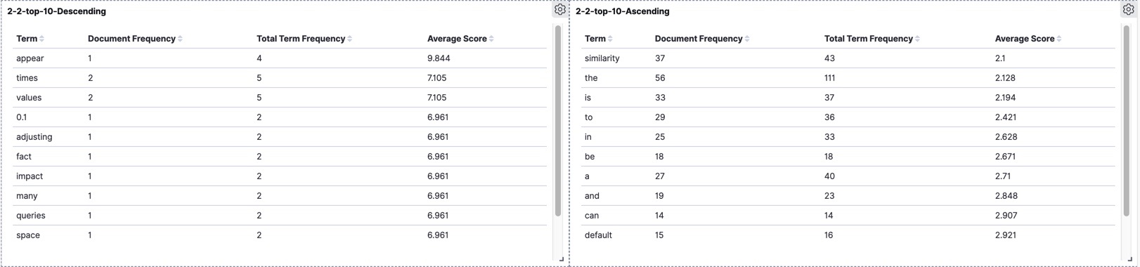
version 6.4
Again "appear" is located on top but none of the terms "times" and "values" even took place in the top ten. In this version, "similarity" and "the" exchanged their spot at the bottom of the table.
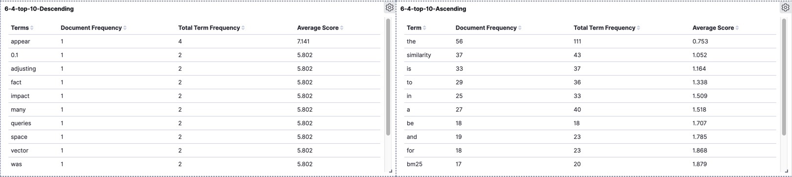
version 7.3
It seems in our dataset the term "appear" truly is the most determinant term when it is present in the query. The tables for versions 6.4 and 7.3 are very close to each other but different from version 2.2.
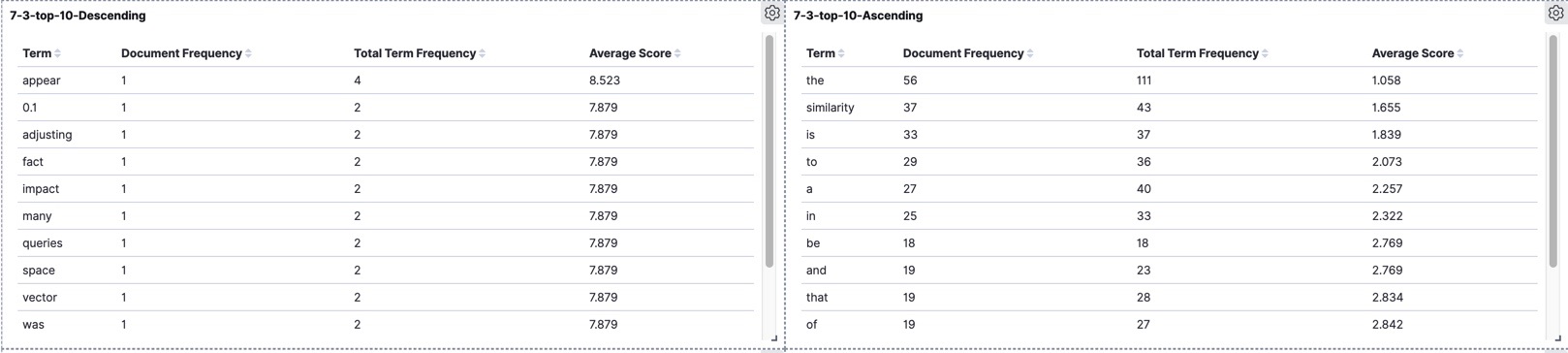
These tables showing, to what extent each individual term in our dataset is important when it is part of the query or in other words, how determinant to be in the process of score calculation. For example, the word “appear” in all three versions got the highest averageScore which means the documents in a match query containing this term would benefit from its higher capability in contributing the final score. On the other hand, we have terms like “the” and “similarity” which are on the bottom of the table and definitely will not play a key role in the score calculation. In the following section, we will use our dataset to show some important factors of the scoring algorithm through different versions.
TF/IDF through different versions
The term rankings vary through different versions of Elasticsearch according to the tables. The very general answer to this variation is the change in the scoring algorithm. To interpret more precisely we will look at the “explain” API of each version with a match query on the term “appear”. The following explain outputs have been pruned to bold out the main concepts.
Version 2.2
By removing the verbose documentation of each component, we can see the contributing elements of the scoring algorithm here.
As we could see in this version alongside tf and idf there is one more element which is called "fieldNorm". This factor is calculated in the indexing time.
The longer the field the smaller the value.
In other words, it makes sure that the shorter fields contribute more to the final score.
More details about the equation of each component could be found here.
{
   "_explanation": {
      "description": "weight(text:appear in 81) [PerFieldSimilarity], result of:",
      "details": [
         {
            "description": "fieldWeight in 81, product of:",
            "details": [
               {
                  "description": "tf(freq=4.0), with freq of: (freq)"
               },
               {
                  "description": "idf(docFreq=1, maxDocs=101)"
               },
               {
                  "description": "fieldNorm(doc=81)"
               }
            ]
         }
      ]
   }
}
There are some missing contributors of the algorithm in this example because there are not enough terms in the query to show their impact in the score calculation process. One of them that will be explained in the coming sections is "Coordination Factor".
Version 6.4
In this version, tf and idf have kept their impact in the scoring algorithm, although their computation has been changed (the default similarity module in this version is BM25).
{
   "_explanation": {
      "description": "weight(text:appear in 81) [PerFieldSimilarity], result of:",
      "details": [
         {
            "description": "score(doc=81,freq=4.0 = termFreq=4.0\n), product of:",
            "details": [
               {
                  "description": "idf, computed as log(1 + (docCount - docFreq + 0.5) / (docFreq + 0.5)) from:"
               },
               {
                  "description": "tfNorm, computed as (freq * (k1 + 1)) / (freq + k1) from:"
               }
            ]
         }
      ]
   }
}
Version 7.3
Apart from supplementing a boosting factor, the computation of tf is modified in this version compared to version 6.4.
The term dl in this equation stands for document length and avgdl is the average of all document lengths.
It brought back the impact of the "fieldNorm" which was an independent factor in version 2.2, removed in version 6.4 and is part of tf in this version.
No change in the computation of idf from version 6.4 to 7.3.
{
   "_explanation": {
      "description": "weight(text:appear in 81) [PerFieldSimilarity], result of:",
      "details": [
         {
            "description": "score(freq=4.0), product of:",
            "details": [
               {
                  "description": "boost"
               },
               {
                  "description": "idf, computed as log(1 + (N - n + 0.5) / (n + 0.5)) from:"
               },
               {
                  "description": "tf, computed as freq / (freq + k1 * (1 - b + b * dl / avgdl)) from:"
               }
            ]
         }
      ]
   }
}
As seen, all versions have two main concepts in common, tf and idf. The former is the frequency of a term in the document and the later stands for Inverse Document Frequency (generally a reverse relation by the number of documents in which a certain term is contained). Some other factors are involved in the scoring algorithm that varies in versions, like coordination factor. It is missing in this example (for version 2.2) because more than one clause (or term) is required to have it involved. We will take a look at it with another example. This factor has been removed since Elasticsearch 6.
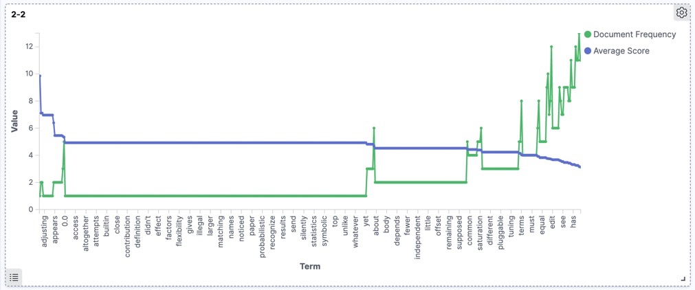
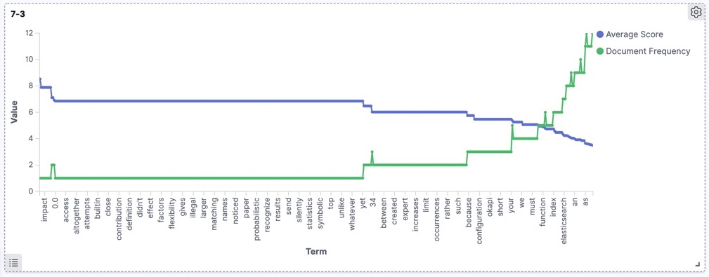
The default for similarity in Elasticsearch 2.2 is known as TF/IDF (detail is here) which is changed from Elasticsearch 5 to BM25 (have a look at Vinh's blog). But according to the main structure of the scoring algorithm, no matter which type of similarity is used, the bigger tf would deliver a bigger score in all versions, the same story is for idf. The difference between similarity modules come from their way of tf and idf calculation. In the older approaches like TF/IDF there is a more direct relation to the number of term frequencies (both in a document and overall documents) but BM25 trying to provide a more mature solution. For example, in TF/IDF the tf is the square of term frequency, which means the more of the same term in a document, the bigger is the tf for it. This approach could overrate the importance of dominant terms which does not let others contribute to the final score. On the other hand, BM25’s diagrams show a raise in the beginning and get stable after a while.
The following diagrams depict the relation of scores and document frequency in different versions for our dataset. As expected generally the same trend is shown by all versions, though the newer versions produce more accurate and cleaner diagrams.
Version 2.2
Version 6.4
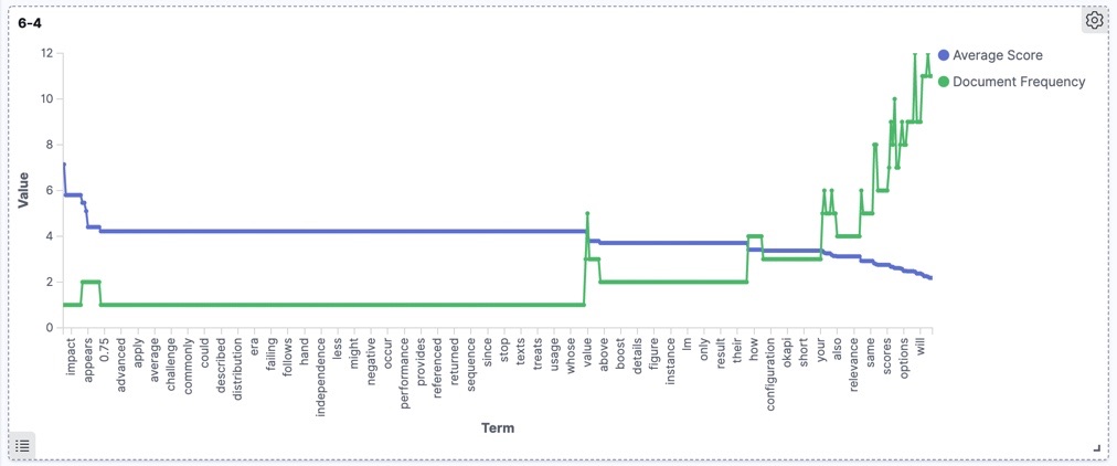
Version 7.3
In the rest of this blog, we will focus on the coordination factor which is removed since Elasticsearch 6. We will see how it could be the source of differences with practical examples.
Coordination Factor
The coordination factor is a score factor based on how many of the query terms are found in the specified document. Quoted from Lucene documentation here. As mentioned, this factor is removed from 6.x onward (more information). This factor does not have any impact on the calculation of tf or idf but had its own role in the scoring equation. That means changing the similarity from BM25 to TF/IDF in version 6 will not bring back this factor into the game again because it has been removed from the main equation. Considering statistics from our dataset, we will do some experiments with the combination of different terms to see how the result set could vary even in such a small dataset.
Statistics are mostly shard based if we want to have the precise comparison, we either use a single shard (not just single node) configuration or the same number of shards in all versions. Having just one shard makes the examination more accurate.
Experiment
In this section, we will run some queries in different versions of Elasticsearch to show the differences by coordination factor. To that end, we have to design a match query with a couple of terms. Let’s start with a single term where the coordination factor would not be in charge because the final query will have just one clause.
query : “algorithm”
| rank | Version 2.2 | Version 6.4 | Version 7.3 |
|---|---|---|---|
| 1 | 59 (~4.69) | 59 (~3.26) | 59 (~4.43) |
| 2 | 64 (~4.69) | 64 (~3.26) | 64 (~4.43) |
| 3 | 94 (~4.69) | 94 (~3.26) | 94 (~4.43) |
| 4 | 25 (~3.32) | 25 (~2.37) | 25 (~3.85) |
| 5 | 33 (~3.32) | 33 (~2.37) | 33 (~3.85) |
| 6 | 66 (~3.32) | 66 (~2.37) | 66 (~3.85) |
| 7 | 72 (~3.32) | 72 (~2.37) | 72 (~3.85) |
| 8 | 74 (~3.32) | 74 (~2.37) | 74 (~3.85) |
| 9 | 79 (~3.32) | 79 (~2.37) | 79 (~3.85) |
The first number is the document ID and the one inside parenthesis depicts the corresponding score. As we could see, there is no difference in rankings in this example among versions.
query : “appear default field similarity”
In this example, we have chosen a combination of terms to expose the differences with presence and absence of coordination factor.
| rank | Version 2.2 | Version 6.4 | Version 7.3 |
|---|---|---|---|
| 1 | 59 (~2.68) | 81 (~3.28) | 81 (~8.52) |
| 2 | 96 (~2.36) | 59 (~3.26) | 59 (~8.42) |
| 3 | 81 (~1.79) | 96 (~3.26) | 96 (~8.08) |
| 4 | 91 (~1.28) | 91 (~2.37) | 91 (~6.46) |
| 5 | 2 (~1.26) | 2 (~2.37) | 2 (~5.54) |
| 6 | 70 (~1.26) | 70 (~2.37) | 70 (~5.54) |
| 7 | 55 (~1.13) | 55 (~2.37) | 55 (~5.14) |
| 8 | 72 (~1.10) | 85 (~2.37) | 85 (~5.02) |
| 9 | 94 (~0.97) | 72 (~2.37) | 95 (~5.02) |
| 10 | 95 (~0.97) | 84 (~3.29) | 97 (~5.02) |
To avoid showing the verbose explain output here for different versions, I will try to explain what happens to the documents with IDs 81 and 59 in this example and why doc 81 appears on top in newer versions but not in 2.2. From the explain output, just the term “appear” is present into doc 81. That means the coordination factor is 0.25 (one out of four) which will be multiplied to the final score in version 2.2 but removed from other versions. Although according to the analysis of our dataset the term “appear” has the biggest tf/idf in all versions, it’s score is multiplied in a small coordination factor because of the absence of other terms in doc 81. In doc 59 all other terms are present but “appear”. According to the statistics from the dataset, the tf/idf for the other terms than "appear" are too small compared to it, but their summation multiplied in 0.75 (three out of four) which provides a bigger score than doc 81 in version 2.2.
Our dataset was a very small one which makes it difficult to show the differences sharply. In the real projects with hundreds of millions of records and each with several lines of text inside, could provide enormous differences in rankings.
Conclusion
Through this blog, we demonstrated practically (in the presence of a small dataset), some differences in scoring algorithms of three different Elasticsearch versions. Sometimes we do a big effort of migration without considering all aspects upfront. Just think we migrate our real data from one version to another and then notice strange behavior in our system because of mismatching numbers. Or completely different result set in the first page for the end-user who had done the same search yesterday. There are some points we should take care of. Never hard code a number derived by the scoring of a specific version because it would not be valid for other versions. If we use parameters in the queries like boosting, they should be re-tuned for newer versions. Sometimes we might also be satisfied with the ranking provided with older versions and want to compensate the impact of breaking changes like removed coordination factor. In those cases, we could use function_score or script_score to simulate the coordination factor.