The Space Between Us - Relevance Scoring with Elasticsearch

June 1, 2019

by Vinh Nguyên

• Elastic Stack

Are we looking for a new home? We also move very soon in to our new office location in Bern. In my previous article about medical use cases, I shortly introduced the capability of geographical distance queries. In this post, we examine its impact on Elasticsearch scoring.

Searching for a new apartment is a challenging task. Search engines can help us to find the right place in the offerings, but IMHO, I have observed some flaws and weak algorithms on existing online solutions. I will get into detail in the following sections.

Elasticsearch is about search. Providing relevant results are our duty as engineers if you use Elasticsearch. I will demonstrate how Elasticsearch overcome these flaws by tuning and administering relevancy for the user.

This article originated from a real-life situation in one of our projects. I take a more joyous example that everybody can relate to the real estate sector. Think of it as you want to find a new apartment for yourself and your family. Thank you to the Job-Room development team by giving me so many opportunities to revisit the exciting parts of a dry theory: The Theory behind Relevance Scoring.

Table of Contents

• Stats for Nerds
• The Data
• Start Searching for Apartments
• Combine Budget Criteria
  • Decay Functions
  • Understanding Score Computation
  • Combine Function Scores
  • Tweaking Score
• Going The Extra Mile
• Summary

Stats for Nerds

• Time Spent: 3 hours 23 minutes
• The Space Between Us is the title of a movie.
• Most-played song: Our House by Madness
• The Gaussian distribution is named after the mathematician Carl Friedrich Gauß.
• All examples are for Elasticsearch v7.1.0. The mapping type is deprecated and not needed anymore.

The Data

Let us look into some data.

We put all rental information in the index rentals and define all essential properties that are not text.

curl -XPUT "http://localhost:9200/rentals" -H 'Content-Type: application/json' -d'
{
  "mappings": {
    "properties": {
      "rooms": {
        "type": "float"
      },
      "size": {
        "type": "integer"
      },
      "public-transport": {
        "type": "integer"
      },
      "price": {
        "type": "integer"
      },
      "address": {
        "properties": {
          "location": {
            "type": "geo_point"
          },
          "zipcode": {
            "type": "integer"
          },
          "city": {
            "type": "keyword"
          }
        }
      }
    }
  }
}'

I have some example data. Run this against your Elasticsearch endpoint.

curl -XPOST "http://localhost:9200/_bulk" -H 'Content-Type: application/json' -d'
{"index":{"_index":"rentals","_id":"21322197"}}
{"title":"4.5-Zimmerwohnung im Stadtzentrum","rooms":4.5,"size":125,"public-transport":20,"price":1990,"address":{"location":"47.143299, 7.248760","zipcode":2502,"city":"Biel"}}
{"index":{"_index":"rentals","_id":"21321999"}}
{"title":"4 1/2 Zimmer Wohnung","rooms":4.5,"size":125,"public-transport":100,"price":1790,"address":{"location":"47.123707, 7.281259","zipcode":2555,"city":"Brügg"}}
{"index":{"_index":"rentals","_id":"21321337"}}
{"title":"Moderne 3.5 Zimmerwohnung ","rooms":3.5,"size":85,"public-transport":400,"price":2100,"address":{"location":"47.016240, 7.482030","zipcode":3302,"city":"Moosseedorf"}}
{"index":{"_index":"rentals","_id":"21304252"}}
{"title":"Grosszügige 4,5 Zimmer Wohnung","rooms":4.5,"size":120,"public-transport":350,"price":1980,"address":{"location":"47.073559, 7.305770","zipcode":3250,"city":"Lyss"}}
{"index":{"_index":"rentals","_id":"21302806"}}
{"title":"Grosszügige 4,5 Zimmer Wohnung","rooms":4.5,"size":107,"public-transport":100,"price":2390,"address":{"location":"46.947975, 7.447447","zipcode":3008,"city":"Bern"}}
{"index":{"_index":"rentals","_id":"21296614"}}
{"title":"Grosse 5,5 Zimmerwohnung im Erdgeschoss an ruhiger Lage","rooms":5.5,"size":147,"public-transport":130,"price":1980,"address":{"location":"47.192829, 7.395120","zipcode":2540,"city":"Grenchen"}}
{"index":{"_index":"rentals","_id":"21261864"}}
{"title":"Moderne 4.5-Zimmer-Whg","rooms":4.5,"size":115,"public-transport":500,"price":2350,"address":{"location":"47.038050, 7.376610","zipcode":3054,"city":"Schüpfen"}}
{"index":{"_index":"rentals","_id":"21320202"}}
{"title":"Wohnung mit toller Aussicht","rooms":3.5,"size":84,"public-transport":500,"price":2070,"address":{"location":"46.956170, 7.482840","zipcode":3072,"city":"Ostermundigen"}}
{"index":{"_index":"rentals","_id":"21264148"}}
{"title":"Wo sich Fuchs und Hase Gute Nacht sagen","rooms":4.5,"size":89,"public-transport":100,"price":1795,"address":{"location":"46.998320, 7.451090","zipcode":3072,"city":"Zollikofen"}}
'

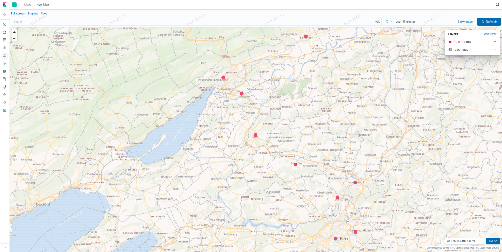
That is our data on a Coordinate Map in Kibana.

Start Searching for Apartments

In the first query, we are searching for apartments that match our first criteria:

• We need at least three rooms, but we would favour apartments with four rooms.
• Apartments with four rooms get a boost of 1.

Most Elasticsearch users don't know the yaml output option. I find it more readable for our example, and we can distinguish better queries (JSON) from results (YAML).

GET rentals/_search?format=yaml
{
  "_source": ["title", "rooms"],
  "query": {
    "bool": {
      "should": [
        { "range": { "rooms": { "gte": 3 }}},
        { "range": { "rooms": { "gte": 4, "boost": 1 }}}
      ]
    }
  }
}

The relevant output in YAML format:

---
hits:
  total:
    value: 9
    relation: "eq"
  max_score: 2.0
  hits:
  - _index: "rentals"
    _type: "_doc"
    _id: "21322197"
    _score: 2.0
    _source:
      rooms: 4.5
      title: "4.5-Zimmerwohnung im Stadtzentrum"
  - _index: "rentals"
    _type: "_doc"
    _id: "21321999"
    _score: 2.0
    _source:
      rooms: 4.5
      title: "4 1/2 Zimmer Wohnung"
  - ... many more documents
  - _index: "rentals"
    _type: "_doc"
    _id: "21321337"
    _score: 1.0
    _source:
      rooms: 3.5
      title: "Moderne 3.5 Zimmerwohnung "
  - _index: "rentals"
    _type: "_doc"
    _id: "21320202"
    _score: 1.0
    _source:
      rooms: 3.5
      title: "Wohnung mit toller Aussicht"

As you can see, if a document matches the non-textual criteria, the document gets a _score of 1.0. All documents that also matches the requirements of four rooms get a boost of 1 and the result score is 2.0. So documents with a higher score get ranked first.

| rank | rooms | city          | score |
| ---- | ----- | ------------- | ------|
| 1    | 4.5   | Biel          | 2.0   |
| 2    | 4.5   | Brügg         | 2.0   |
| 3    | 4.5   | Lyss          | 2.0   |
| 4    | 4.5   | Bern          | 2.0   |
| 5    | 4.5   | Grenchen      | 2.0   |
| 6    | 5.5   | Schüpfen      | 2.0   |
| 7    | 4.5   | Zollikofen    | 2.0   |
| ==== | ===== | ============= | ===== |
| 8    | 3.5   | Moosseedorf   | 1.0   |
| 9    | 3.5   | Ostermundigen | 1.0   |

Combine Budget Criteria

The previous section gave us the idea of how relevancy is achieved by scoring. Real life searches aren't limited to one criterion. They often consist of various aspects.

In the next query, we look into another critical criterion, the rental fee or price. We combine them with our previous search. Don't be shocked, looking at the monthly rental fees in our data. That is pretty normal in Switzerland.

• We switch to the function_score, that allows you to modify the score of documents that are retrieved by a query.
• We keep our room preferences.

The price reflects another user desire. If your budget is not unlimited, you would probably prefer something in your budget above something expensive. For the price field, the origin would be 1700 CHF, and the scale depends on how much you are willing to pay additionally, for example, 300 CHF. This budget is not necessarily your limit but gives us a very sensible ranking.

GET rentals/_search?format=yaml
{
  "_source": [
    "address.city",
    "rooms",
    "price"
  ],
  "query": {
    "function_score": {
      "query": {
        "bool": {
          "should": [
            { "range": { "rooms": { "gte": 3 } } },
            { "range": { "rooms": { "gte": 4, "boost": 2 } } }
          ]
        }
      },
      "functions": [
        { "gauss": { "price": { "origin": "1700", "scale": "300" } } }
      ]
    }
  }
}

The simplified output in YAML:

---
hits:
  max_score: 2.8185682
  hits:
  - _id: "21321999"
    _score: 2.8185682
    _source:
      rooms: 4.5
      address:
        city: "Brügg"
      price: 1790
  - _id: "21264148"
    _score: 2.7985601
    _source:
      rooms: 4.5
      address:
        city: "Zollikofen"
      price: 1795
  - _id: "21304252"
    _score: 1.6401769
    _source:
      rooms: 4.5
      address:
        city: "Lyss"
      price: 1980
  - _id: "21296614"
    _score: 1.6401769
    _source:
      rooms: 5.5
      address:
        city: "Grenchen"
      price: 1980
  - _id: "21322197"
    _score: 1.5697317
    _source:
      rooms: 4.5
      address:
        city: "Biel"
      price: 1990
  - _id: "21320202"
    _score: 0.34841746
    _source:
      rooms: 3.5
      address:
        city: "Ostermundigen"
      price: 2070
  - _id: "21321337"
    _score: 0.29163226
    _source:
      rooms: 3.5
      address:
        city: "Moosseedorf"
      price: 2100
  - _id: "21261864"
    _score: 0.115865104
    _source:
      rooms: 4.5
      address:
        city: "Schüpfen"
      price: 2350
  - _id: "21302806"
    _score: 0.07667832
    _source:
      rooms: 4.5
      address:
        city: "Bern"
      price: 2390

Decay Functions

That looks nice. However, what happened behind the curtains? Let us look closer to the scores.

| rank   | price in CHF | rooms  | city             | score        |
| ------ | ------------ | ------ | ---------------- | ------------ |
| 1      | 1790         | 4.5    | Brügg            | 2.8185682    |
| 2      | 1795         | 4.5    | Zollikofen       | 2.7985601    |
| ====== | ============ | ====== | ================ | ============ |
| 3      | 1980         | 4.5    | Lyss             | 1.6401769    |
| 4      | 1980         | 5.5    | Grenchen         | 1.6401769    |
| 5      | 1990         | 4.5    | Biel             | 1.5697317    |
| ====== | ============ | ====== | ================ | ============ |
| 6      | 2070         | 3.5    | Ostermundigen    | 0.34841746   |
| 7      | 2100         | 3.5    | Moosseedorf      | 0.29163226   |
| 8      | 2350         | 4.5    | Schüpfen         | 0.115865104  |
| 9      | 2390         | 4.5    | Bern             | 0.07667832   |

At the start of the table, prices get clustered together at the top, and that there isn't a significant gap in the score between apartments that varies from the origin 1700.

At some point, it starts severely penalizing apartments, which are farther away from the origin but still on the scale of 300.

Finally, we want apartments outside our preferred range to bottom out at some point.

This decay separates our results into three neat compartments with a very natural transition between all three parts.

1. Apartments, that farther it gets from the origin price, receive a minor penalty or decay.
2. Moderately more expensive apartments get a more substantial score penalty, increasing more and more within the scale.
3. Apartments outside our preferred range get a severe punishment.

Decay functions score a document with a function that decays depending on the distance of a numeric field value of the document from a user given origin.

Elasticsearch has three types of curves for dealing with decays, gauss, exp(onential), and linear.

We have used the Gauss decay in the above example. In most scenarios, the gauss type is the most useful one. We will deal with the use cases for the other decay functions in future blog posts.

Understanding Score Computation

One of the challenges for super curious people is to trace the score computation. You can always add the explain option to the query.

For instance, the following query returns only 1 document to check the score of 2.8185682.

GET rentals/_search?format=yaml
{
  "size": 1,
  "_source": ["address.city","rooms","price"],
  "query": {
    "function_score": {
      "query": {
        "bool": {
          "should": [
            { "range": { "rooms": { "gte": 3 } } },
            { "range": { "rooms": { "gte": 4, "boost": 2 } } }
          ]
        }
      },
      "functions": [
        { "gauss": { "price": { "origin": "1700", "scale": "300" } } }
      ]
    }
  },
  "explain": true
}

This will give us in detail the formula:

---
hits:
  total:
    value: 9
    relation: "eq"
  max_score: 2.8185682
  hits:
  - _shard: "[rentals][0]"
    _node: "uJudeEy4QmmCznWNxU4Eqg"
    _index: "rentals"
    _type: "_doc"
    _id: "21321999"
    _score: 2.8185682
    _source:
      rooms: 4.5
      address:
        city: "Brügg"
      price: 1790
    _explanation:
      value: 2.8185682
      description: "function score, product of:"
      details:
      - value: 3.0
        description: "sum of:"
        details:
        - value: 1.0
          description: "rooms:[1077936128 TO 2139095040]"
          details: []
        - value: 2.0
          description: "rooms:[1082130432 TO 2139095040]^2.0"
          details: []
      - value: 0.93952274
        description: "min of:"
        details:
        - value: 0.93952274
          description: "Function for field price:"
          details:
          - value: 0.93952274
            description: "exp(-0.5*pow(MIN[Math.max(Math.abs(1790.0(=doc value) -\
              \ 1700.0(=origin))) - 0.0(=offset), 0)],2.0)/64921.27684000335)"
            details: []
        - value: 3.4028235E38
          description: "maxBoost"
          details: []

That can be very confusing at first sight, but it is effortless to understand.

• The _score is a product (that means we have a multiplication).
• 3.0 is the value of the rooms search.
• 0.93952274 is the result of the function decay. The default decay is 0.5, as seen in the description formula.
• 3.0 x 0.93952274 = 2.8185682 is the final score.

Combine Function Scores

In the previous section, you had a first glimpse of the function score. In this section, I will demonstrate how to combine function scores.

Remember that I said that I had experienced flaws in the search results of real estate portals. No portal to my knowledge has an adequate relevancy scoring based on the location.

The most important thing I have learned looking for a property is the location. The location is the only thing you can not change about an apartment or house.

Let us assume I have switched my working location. Now I want to find a new apartment based on my new working site in a 20 km radius. Now we add another influence to our ranking: the location. My new origin is Lyss, a very family-friendly city, and my scale is 5 kilometres. We do a function score on a geo_point field and our scale is defined as 5 km radius (see pictures below).

GET rentals/_search
{
  "query": {
    "function_score": {
      "query": {
        "bool": {
          "should": [
            { "range": { "rooms": { "gte": 3 } } },
            { "range": { "rooms": { "gte": 4, "boost": 1 } } }
          ]
        }
      },
      "functions": [
        { "gauss": { "price": { "origin": "1700", "scale": "300" } } },
        { "gauss": {
            "address.location": {
              "origin": "47.073560, 7.305770",
              "scale": "5km"
            }
          }
        }
      ],
      "score_mode": "multiply"
    }
  }
}

• The new gauss function on the location is similar to the geo_distance query.
• We want to multiply the scores to get a ranking based on price and location.

We get these results:

| rank   | price in CHF | rooms  | city            | distance | score          |
| ------ | ------------ | ------ | --------------- | -------- | -------------- |
| 1      | 1980         | 4.5    | Lyss            |     0 km | 1.0934513      |
| 2      | 1790         | 4.5    | Brügg           |     7 km | 0.7212604      |
| 3      | 1990         | 4.5    | Biel            |    10 km | 0.117894106    |
| ====== | ============ | ====== | =============== | ======== | ============== |
| 4      | 2350         | 4.5    | Schüpfen        |     8 km | 0.022560354    |
| 5      | 1795         | 4.5    | Zollikofen      |    16 km | 0.009281355    |
| 6      | 2540         | 5.5    | Grenchen        |    17 km | 0.0023489068   |
| ====== | ============ | ====== | =============== | ======== | ============== |
| 7      | 2100         | 3.5    | Moosseedorf     |    16 km | 6.728557E-4    |
| 8      | 2070         | 3.5    | Ostermundigen   |  21.5 km | 2.0915837E-5   |
| 9      | 2390         | 4.5    | Bern            |  20.5 km | 9.355606E-6    |

As you can see, the price is not an essential criterion anymore. Lyss got a higher score, due to distance equals 0, but it has a higher rent than the second rank in Brügg.

Tweaking Score

Now we have two function scores on price and location. If you favour price more than the place, you can tweak the decay of the location score.

{
  "gauss": {
    "address.location": {
      "origin": "47.073560, 7.305770",
      "scale": "5km",
      "offset": "10km",
      "decay": 0.25
    }
  }
}

Our new tweak in detail:

• If an offset is defined, the decay function will only compute the decay function for documents with a distance more significant than the specified offset, i. e. apartments don't get a penalty if there are within 10 km radius. This reflects our motivation to look in a 20 km radius, but we favour locations in half that range.
• The scale of 5 km will be applied after the 10 km radius offset.
• I use a lower decay offset of 0.25 instead of the default 0.50 for location, and the new results are more in favour of the price now.

Our new results:

| rank   | price in CHF | rooms  | city            | distance | score          |
| ------ | ------------ | ------ | --------------- | -------- | -------------- |
| 1      | 1790         | 4.5    | Brügg           |     7 km | 1.8790455      |
| 2      | 1980         | 4.5    | Lyss            |     0 km | 1.0934513      |
| 3      | 1990         | 4.5    | Biel            |    10 km | 1.0464878      |
| ====== | ============ | ====== | =============== | ======== | ============== |
| 4      | 1795         | 4.5    | Zollikofen      |    16 km | 0.82701206     |
| 5      | 2540         | 5.5    | Grenchen        |    17 km | 0.29112878     |
| ====== | ============ | ====== | =============== | ======== | ============== |
| 6      | 2100         | 3.5    | Moosseedorf     |    16 km | 0.081350505    |
| 7      | 2350         | 4.5    | Schüpfen        |     8 km | 0.0772434      |
| 8      | 2070         | 3.5    | Ostermundigen   |  21.5 km | 0.005118213    |
| 9      | 2390         | 4.5    | Bern            |  20.5 km | 0.0020463988   |

You can see that the score is less extreme and we have some switches in the ranking. Now the distance of our origin has less weight than before, and Brügg is again at the top of the search results.

In conclusion:

• The function_score is very easy to use in conjunction with relevance scoring.
• You can combine as many function scores as you want.
• Many function scores will create a significant tax to your query performance.
• So choose a reasonable trade-off between what is essential and what not regarding performance.

You could also take into consideration:

• the size in square meters of the apartment
• the nearest distance to the next public transportation

Relevant scores are a good start and an excellent baseline to rule out many options. From my experience sometimes even the most mathematical scores do not contribute to the solution if your better half disagrees or dislikes the place. Other factors, like the neighbourhood, education, the entertainment offering (no Salsa dance club) and many more reasons can come into play.

Going The Extra Mile

As you can see, the distance is significant for the apartment choice. Sometimes it can be misleading or be a red herring. Distance is in no correlation to the time you spend travelling from your home to your working place. No rental portal provides a feature to uncover or illustrate the relationship between distance and travelling time.

As always, you can quickly build your solutions on top of Elasticsearch. In the next picture, you can see a 20 kilometres radius around Lyss, the working place. I correlate that to a travelling time of one hour with public transportation.

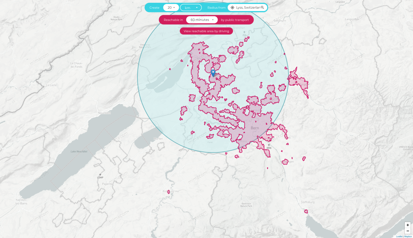
13% of the 60 minutes public transport time area falls beyond the radius, i.e. cities like Fribourg, Münsingen or Thun, have an excellent connection. These cities could be equally eligible for our new home. They aren't in the radius but within the transport time.

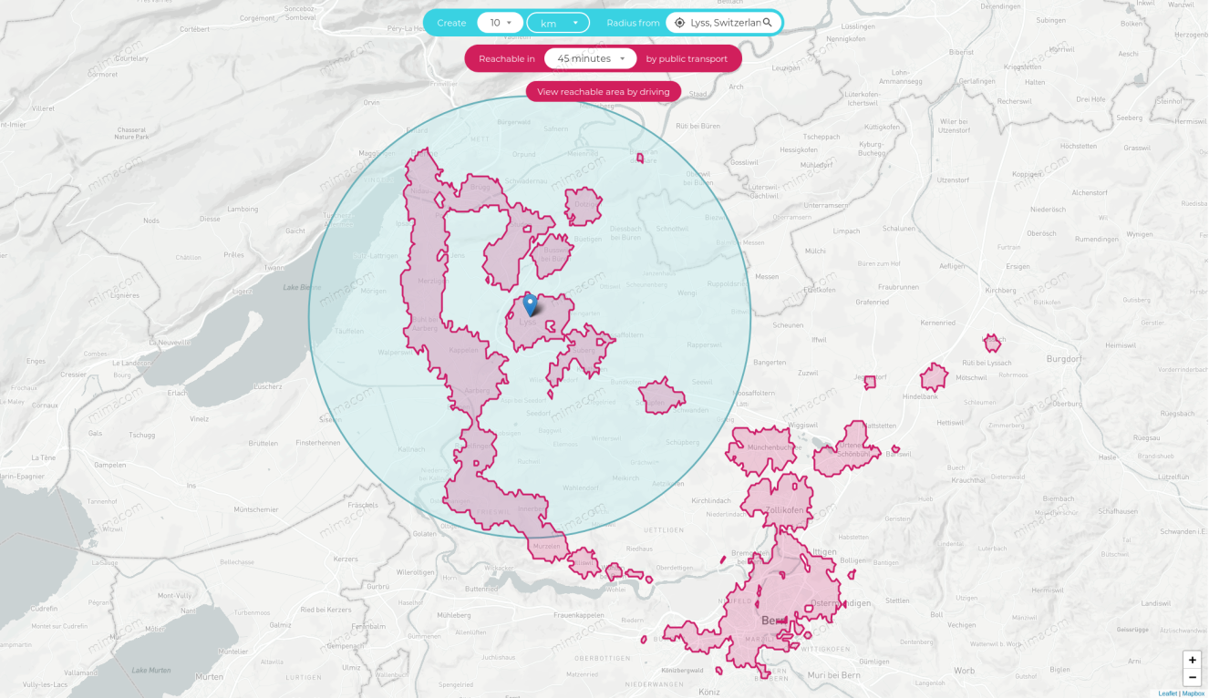
If you narrow it down to 10 kilometres and only 45 minutes travelling time, you see that still, 41% of the 45 minutes public transport time area falls beyond the radius. So rather than focusing on simple distances, we should take the travelling time and train frequency into consideration.

Summary

You have learned in this article:

• A small example of how scores express relevance.
• How to impact rankings with function scores.
• A decay function uses penalty to filter out less relevant documents.
• How to combine multiple function scores.
• How to accomplish consistent hits with simple tweaking of the function_score query.
• Results are only an orientation.
• The final decision in moving is mostly made by your stakeholders :-).

If you like to know more or disagree, don't hesitate to put a comment below. We are open to hear your point of view or happy to help you if you might need assistance in relevance scoring.