Predicting Hike Times with Machine Learning
Introduction
In Switzerland, for most hiking destinations signs are showing rough time estimates, so that people know how long it will take to reach the next peak or mountain hut.
Alpine clubs use a standardised approach to predict these times.
The underlying formulas are tailored for slower hikers intentionally.
This conservative approach is to prevent inexperienced hikers from ending up in distress in the mountains.

DIN 33466 norms the formula to be used to calculate the distances and is the base for signalisation in the German-speaking parts of the Alps and also in Slovenia.
According to DIN 33466 a hiker can cover the following distances within one hour - 300 m of uphill, 500 m of downhill, 4 km of distance.
Times for vertical and horizontal movement are calculated separately and half of the smaller value is added to the larger one to determine the total movement time required.
The Swiss Alpine Club (SAC) uses a slightly simpler formula in its handbook (Winkler, Brehm, Haltmeier; Bergsport Sommer: Technik, Taktik, Sicherheit (2010); SAC-Verlag), which says that a hiker covers 4 km in distance per hour or 400 m of uphill per hour.
Depending on the terrain an additional hour can be added for each 800 m of downhill.
# Python3
def din33466(uphill, downhill, distance):
    vertical = downhill / 500.0 + uphill / 300.0
    horizontal = distance / 4.0
    return min(vertical, horizontal) / 2 + max(vertical, horizontal)

def sac(uphill, downhill, distance):
    return uphill/400.0 + distance/4.0

for hike in ((900, 300, 8), (1500, 500, 20)):
    t1 = din33466(*hike)
    t2 = sac(*hike)
    print("Hike time for {} m of uphill, {} m of downhill and a distance of {} km".format(*hike))
    print("according to {0:>10}: {1:>8.2f} h".format("DIN33466", t1))
    print("according to {0:>10}: {1:>8.2f} h".format("SAC", t2))
Hike time for 900 m of uphill, 300 m of downhill and a distance of 8 km
according to   DIN33466:     4.60 h
according to        SAC:     4.25 h

Hike time for 1500 m of uphill, 500 m of downhill and a distance of 20 km
according to   DIN33466:     8.50 h
according to        SAC:     8.75 h
More experienced hikers can substitute the values in these formulas to get results which fit their personal fitness level - or use machine learning.
Let's do the latter and show how machine learning can be used to achieve better results.
Structure
Data scientists often find themselves spending much time with data acquisition and preparation (in the 2017 Kaggle survey "dirty data" was ranked the highest barrier, A Glimpse into The Daily Life of a Data Scientist), yet most tutorials start with ready to use datasets. This time we start with nothing but a simple problem and gather the data ourselves to provide insight into the process from data gathering to model creation.
The first part demonstrates how data which is publicly available in the Web can be scraped and prepared using Scrapy, a Python library which makes building crawlers quite easy.
In the second part, we use our gathered data to build different machine learning models with sklearn and keras to predict the hike time and evaluate them against a held-out test dataset.
Part 1: Data Gathering
With a small self-build web crawler, we fetch an initial set of GPS recorded tracks as GPX files from hikr.org.
Hikr.org is an online platform where users can upload their tracks and write tour reports.
GPX (GPS Exchange Format) is an XML based format for storing waypoints, tracks and routes.
The crawled GPX files are then processed to extract features such as minimum and maximum altitude, geographic bounds, track length, uphill and downhill.
Building a spider with Scrapy
The steps needed to fetch a GPX file from hikr.org are as follows:
- search for all hiking reports
- for all found reports:
- open a report detail page
- if a GPX file is attached to the report, download it
On hikr.org authentication is not required to download files and no captchas have to be solved to perform these steps, thus automating this was straightforward and the resulting class fits on a few lines of code as shown below.
import scrapy

class GpxSpider(scrapy.Spider):
    name = 'gpx'
    start_urls = ['http://www.hikr.org/filter.php?act=filter&a=ped&ai=100&aa=630']

    def parse(self, response):
        for href in response.css('.content-list a::attr(href)'):
            yield response.follow(href, self.parse_detail_page)

        # follow pagination links
        for href in response.css('a#NextLink::attr(href)'):
            yield response.follow(href, self.parse)

    def parse_detail_page(self, response):
        gpx_href = [href for href in response.css('#geo_table a::attr(href)').extract() if href.endswith(".gpx")]
        if len(gpx_href) >= 1:
            yield {
                'file_urls': [gpx_href[0]],
                'difficulty': response.xpath(
                    'normalize-space(//td[normalize-space() ="Hiking grading:"]/following-sibling::td/a/text())').extract_first(),
                'user': response.css('.author a.standard::text').extract_first(),
                'name': response.css('h1.title::text').extract_first(),
                'url': response.url
            }
In the class above, the parse method is called with the responses of the requests to all URLs defined
in the start_urls array.
In this case, this is only one URL which points to the list view with all hiking reports.
We are interested in two links on the overview page - the link to a detail page of a report, and the link to the next page of results.
By yielding response.follow(href, handler) we instruct Scrapy to send a request to the URL and
call the handler with the response of that request.
The detail page is handled by parse_detail_page which extracts the difficulty rating of the hike, username, report name and URL.
By yielding a dictionary, we tell Scrapy to persist these values.
The file_urls field only contains the link to the GPX file that we want to fetch.
By adding the Files Pipeline in the Scrapy settings,
the URLs listed in this field will be fetched and stored automatically, and the file path is added to the output dictionary.
The following configuration entry has to be present in settings.py to enable the Files Pipeline:
ITEM_PIPELINES = {
   'scrapy.pipelines.files.FilesPipeline': 300,
}
FILES_STORE = 'downloads'
After the crawler had been run for several hours, a few thousand entries were stored in a text file in JSON Lines format.
There are some things to keep in mind when using Scrapy:
- You can (and should) test your code in the interactive Scrapy shell. This is especially useful to quickly find good CSS or xpath selectors without running the spider.
- Enable throttling. You don't want to cause a denial of service by bombarding your target with thousands of requests.
- Only crawl a small amount in the beginning and verify that the collected data works for your problem. The earlier potential issues can be discovered, the better.
- If the API or website has rate limits, consider starting the job with job persistence enabled so you can pause and continue later. Alternatively consider using a mesh proxy provider to distribute your requests over several IPs.
Processing GPX files with gpxpy and writing track information to MongoDB
It was assumed that length, uphill and downhill distance are the most important attributes to be extracted from the GPX files.
Obviously the time in movement needed to be determined as well as this is the feature that our models should predict.
The library gpxpy was used to parse the downloaded GPX files and calculate these features.
Instead of writing the results back to a text file, they were inserted into MongoDB (mainly for demonstration purposes).
With the given amount of data this was not strictly necessary, however with larger datasets one can benefit from querying and indexing capabilities of databases to train models with batches of data.
A CLI import script was built to do the processing and insertion of result batches into MongoDB.
./mongo_import.py -c tracks -i tracks.jl
The import script fetches a batch of tracks from the JSON lines file, processes the entries with gpxpy and then bulk inserts the extracted track information to MongoDB.
The source code of the import script is available here.
The created dataset has also been made available as a CSV file on kaggle.com/roccoli/gpx-hike-tracks.
Part 2: Building Models to predict hike times
We load the dataset that we have previously created and start with some basic analysis to understand the nature of the data.
import json
from pymongo import MongoClient
import gpxpy
import pandas as pd
from matplotlib import pyplot
%matplotlib

mongo_uri = "mongodb://localhost:27017"
mongo_db = "tracks"
mongo_collection = "hikr"

client = MongoClient(mongo_uri)
db = client[mongo_db]
collection = db[mongo_collection]
Loading the dataset into a dataframe
For further processing we load all tracks from the collection into a pandas dataframe.
# fetch a single document
track = collection.find_one(projection={"gpx": 0, "url": 0, "bounds": 0, "name": 0})
values = [track.values() for track in collection.find(projection={"gpx": 0, "url": 0, "bounds": 0, "name": 0})]
# we later use track document's field names to label the columns of the dataframe
df = pd.DataFrame(columns=track.keys(), data=values).set_index("_id")
The difficulty column contains category data as strings.
As most models won't work with text values, we can extract the second character which results in an ordinal encoding.
For categorical data, which cannot be transformed that easily, there are some builtin helpers like the sklearn CategoricalEncoder or the Keras one-hot-encoding function.
df['avg_speed'] = df['length_3d']/df['moving_time']
df['difficulty_num'] = df['difficulty'].map(lambda x: int(x[1])).astype('int32')
Removing Outliers
Looking at min and max values it is apparent that there are some tracks which we want to exclude from our dataset.
An infinite average speed, or a min elevation of more than 30km below sea level just don't seem right.
We can remove the extremes at both sides and remove all rows where there are null values.
df.describe()
| max_speed | downhill | max_elevation | uphill | length_3d | moving_time | min_elevation | |
|---|---|---|---|---|---|---|---|
| count | 12141.000000 | 12141.000000 | 10563.000000 | 12141.000000 | 1.214100e+04 | 12141.000000 | 10563.000000 |
| mean | 1.746356 | 879.145539 | 1934.281708 | 942.184362 | 1.874771e+04 | 12848.445268 | 1003.331150 |
| std | 5.394065 | 1028.618856 | 784.968353 | 1065.498993 | 4.093098e+05 | 11599.792248 | 813.001041 |
| min | 0.000000 | 0.000000 | -1.000000 | 0.000000e+00 | 0.000000e+00 | 0.000000 | -32768.000000 |
| 25% | 1.078841 | 256.519000 | 1382.275000 | 420.142000 | 8.254129e+03 | 5260.000000 | 560.020000 |
| 50% | 1.367020 | 823.199002 | 1986.700000 | 882.000000 | 1.200577e+04 | 12990.000000 | 960.090000 |
| 75% | 1.604181 | 1266.923000 | 2498.455848 | 1301.005000 | 1.645813e+04 | 18514.000000 | 1389.485000 |
| max | 192.768748 | 52379.200000 | 5633.462891 | 35398.006781 | 3.189180e+07 | 189380.000000 | 4180.000000 |
# drop na values
df.dropna()
df = df[df['avg_speed'] < 2] # an avg of > 2m/s is probably not a hiking activity
df = df[df['min_elevation'] > 0]
df = df[df['length_2d'] < 100000]
Correlations
We expect altitude changes and track distance to be highly correlated with the moving time as these two features are also used in the formulas used by the alpine clubs. However there might be other features which correlate with moving time and may be good candidates for our models. The chart below shows the Pearson correlation values.
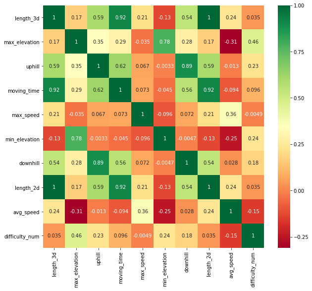
As expected, changes in altitude and distance have the highest correlations with moving time.
Max elevation also shows low correlation as the terrain in higher altitudes can be more challenging than in lower altitudes.
Interestingly the difficulty score doesn't seem to correlate much with the moving time.
This might be due to several reasons: The difficulty score of a whole tour is based on the most difficult section, it is set by users and thus varies due to subjectivity.
Also a difficult track may be exposed and only suitable for experienced hikers, but it is not automatically terrain which slows one down.
Building the models
Before putting too much time into a sophisticated model it is important to develop a simple baseline. Any other model can then be benchmarked against it. For many problems these simple baselines are already hard to beat and allow to identify approaches which can be discarded early.
A strong baseline
Given the simple nature of the problem, we will use a linear regression model to predict the moving time based on the most correlated fields (length_3d, uphill, downhill and max_elevation).
from sklearn.linear_model import LinearRegression
from sklearn.model_selection import train_test_split
from sklearn.preprocessing import Normalizer
from sklearn.metrics import r2_score
from sklearn.metrics import mean_squared_error

y = df.reset_index()['moving_time']
x = df.reset_index()[['downhill', 'uphill', 'length_3d', 'max_elevation']]

x_train, x_test, y_train, y_test = train_test_split(x, y, test_size=0.20, random_state=42)

lr = LinearRegression()
lr.fit(x_train, y_train)
LinearRegression(copy_X=True, fit_intercept=True, n_jobs=1, normalize=False)
Scikit learn has a list of prebuilt evaluation functions for regression models.
For regression problems, the coefficient of determination ($r^2$) can be used as a measure of how well the regression approximates the real data points.
An ($r^2$) of 1 indicates that the regression predictions perfectly fit the data.
y_pred_lr = lr.predict(x_test)
r2 = r2_score(y_test, y_pred_lr)
mse = mean_squared_error(y_test, y_pred_lr)

print("r2:\t{}\nMSE: \t{}".format(r2, mse))
r2:	0.8277514178527514
MSE: 	9947095.059578164
The coefficient of determination score is already quite high and might be hard to beat using a different model.
Let's compare this against the formula presented in the introduction.
y_pred_sac = df.apply(lambda row : sac(row.uphill, row.downhill, row.length_2d), axis=1)
r2 = r2_score(y, y_pred_sac)
mse = mean_squared_error(y, y_pred_sac)

print("r2:\t{}\nMSE: \t{}".format(r2, mse))
r2:	-2.0866499679137513
MSE: 	201072625.2795519
The formula parameters have not been fitted on our data and thus the results are far from the true values.
GradientBoostingRegressor
Kagglers have successfully applied variants of Gradient Boosting in competitions. This might also be a good fit for our problem.
Gradient boosting is a machine learning technique for regression and classification problems, which produces a prediction model in the form of an ensemble of weak prediction models, typically decision trees.
A good explanation of what Gradient Boosting does can be found in this article.
from sklearn.ensemble import GradientBoostingRegressor
from sklearn.model_selection import train_test_split

gbr = GradientBoostingRegressor(n_estimators=50, random_state=9000)
gbr.fit(x_train, y_train)
GradientBoostingRegressor(alpha=0.9, criterion='friedman_mse', init=None,
             learning_rate=0.1, loss='ls', max_depth=3, max_features=None,
             max_leaf_nodes=None, min_impurity_decrease=0.0,
             min_impurity_split=None, min_samples_leaf=1,
             min_samples_split=2, min_weight_fraction_leaf=0.0,
             n_estimators=50, presort='auto', random_state=9000,
             subsample=1.0, verbose=0, warm_start=False)
y_pred_gbr = gbr.predict(x_test)
r2 = r2_score(y_test, y_pred_gbr)
mse = mean_squared_error(y_test, y_pred_gbr)

print("r2:\t{}\nMSE: \t{}".format(r2, mse))
r2:	0.8516737813634596
MSE: 	8565614.754054507
The GradientBoostingRegressor outperforms our baseline model.
Building a regression model with Keras
Regression models can also be built with neural networks. By not using an activation function in the last layer, the output can be any continuous value (as opposed to a range of 0 to 1 when using i.e. the sigmoid activation).
from keras import Sequential
from keras.optimizers import RMSprop
from keras.layers import Dense, Dropout
from keras.callbacks import EarlyStopping, ModelCheckpoint, ReduceLROnPlateau

model = Sequential()
model.add(Dense(10, input_shape=(4,)))
model.add(Dense(4, input_shape=(4,)))
model.add(Dense(1))
model.compile(optimizer=RMSprop(lr=0.0001), loss='mse')

model.fit(x_train, y_train, epochs=30, batch_size=20, validation_split=0.15, callbacks=[
    ModelCheckpoint(filepath='./keras-model.h5', save_best_only=True),
    EarlyStopping(patience=2),
    ReduceLROnPlateau()
], verbose=0)
model.load_weights(filepath='./keras-model.h5')
y_pred_keras = model.predict(x_test)
r2 = r2_score(y_test, y_pred_keras)
mse = mean_squared_error(y_test, y_pred_keras)

print("r2:\t{}\nMSE: \t{}".format(r2, mse))
r2:	0.8244549079469348
MSE: 	10137463.520027775
This simple Keras model is slightly worse than our baseline model.
Evaluating an ensemble model
The GBR is the strongest model, thus we will weight it higher than our second strongest model. On average the resulting predictions might be closer to the real values.
import numpy as np

combined = (y_pred_keras[:,0] + y_pred_gbr * 2) / 3.0
r2 = r2_score(y_test, combined)
mse = mean_squared_error(y_test, combined)

print("r2:\t{}\nMSE: \t{}".format(r2, mse))
r2:	0.853322624963087
MSE: 	8470396.530372122
The model ensemble gives us a slightly better result.
c = pd.DataFrame([combined, y_test]).transpose()
c.columns = ['combined', 'test']
c['diff_minutes'] = (c['test'] - c['combined']) / 60
c.describe()
| combined | test | diff_minutes | |
|---|---|---|---|
| count | 1824.000000 | 1824.000000 | 1824.000000 |
| mean | 15965.020362 | 16025.400219 | 1.006331 |
| std | 6886.272844 | 7601.326531 | 48.509436 |
| min | 1789.959391 | 239.000000 | -444.008206 |
| max | 86009.021163 | 105431.000000 | 323.699647 |
As can be seen in the table above, the ensemble model performs well for most hikes in our test dataset. However the min and max values indicate that there are a few outliers with predicted times deviating more than 6 hours from the recorded times. These outliers would need special attention if such a model was to be deployed into production.
Limitations and potential improvements
The model is usually only as good as the data it has been trained on. In this case, the dataset that has been used is likely not representative for the majority of hikers. People using a platform like hikr.org are probably hiking on a regular basis and thus might be more trained and faster than the average person. So the results might be biased due to that. There might also be a geographic bias so that results aren't accurate for other geographic areas with different terrain.
While on average the accuracy might be useful, there are still some considerable deviations from the actual values. The results could be improved by grouping people with similar fitness levels and training distinct models for each group. For a new user, a short recorded track could be sufficient to determine which group this user belongs to. Given the group, a more personalised result would be the outcome.
Conclusion
With tools like Scrapy, collecting data from public sources can be done in just a few lines of code.
However, be aware of the limitations - data sources may mainly contain data from a specific type of users.
We could show that a simple linear regression model performed very well for the given task of predicting hike times
which outlines the importance of creating simple baselines.
There are cases where sophisticated machine learning models are not necessary and add complexity to your solution.